ATMI (Atmospheric Impact Simulation) is a project aiming to develop a generic pipeline for the simulation of the atmospheric impact on CMB ground-based experiments. In fact, CMB observations from the ground are strongly limited by the atmosphere: its presence results in both absorption and emission of new signal. Despite the effect of the absorption of the incoming signal is negligible, atmospheric emission constitutes a noise for CMB measurements. This project is divided into several sections, responsable of different tasks:
- Some routines to implement the atmospheric sampling according to the data.
- Reconstruction of the atmospheric model structure, based on the previous sampling.
- Calculations to determine the brightness temperature of the atmosphere, thanks to the am tool (Atmospheric Model - CfA Harvard) for the radiative transfer computation.
Using a collection of data for the atmospheric realizations, it is possible to give a statistic description the behavior of the main variables, such as temperature, pressure and PWV (Precipitable Water Vapour). Those variables are useful to study the homogeneus atmosphere, in order to predict the impact on radiometric measurements. Thanks to the tools provided by this work, the atmospheric variables data can be used in order to describe the statistics and simulate the atmospheric behaviour and how it evolves with time. See atmi for the details about each specific pipeline.
Description
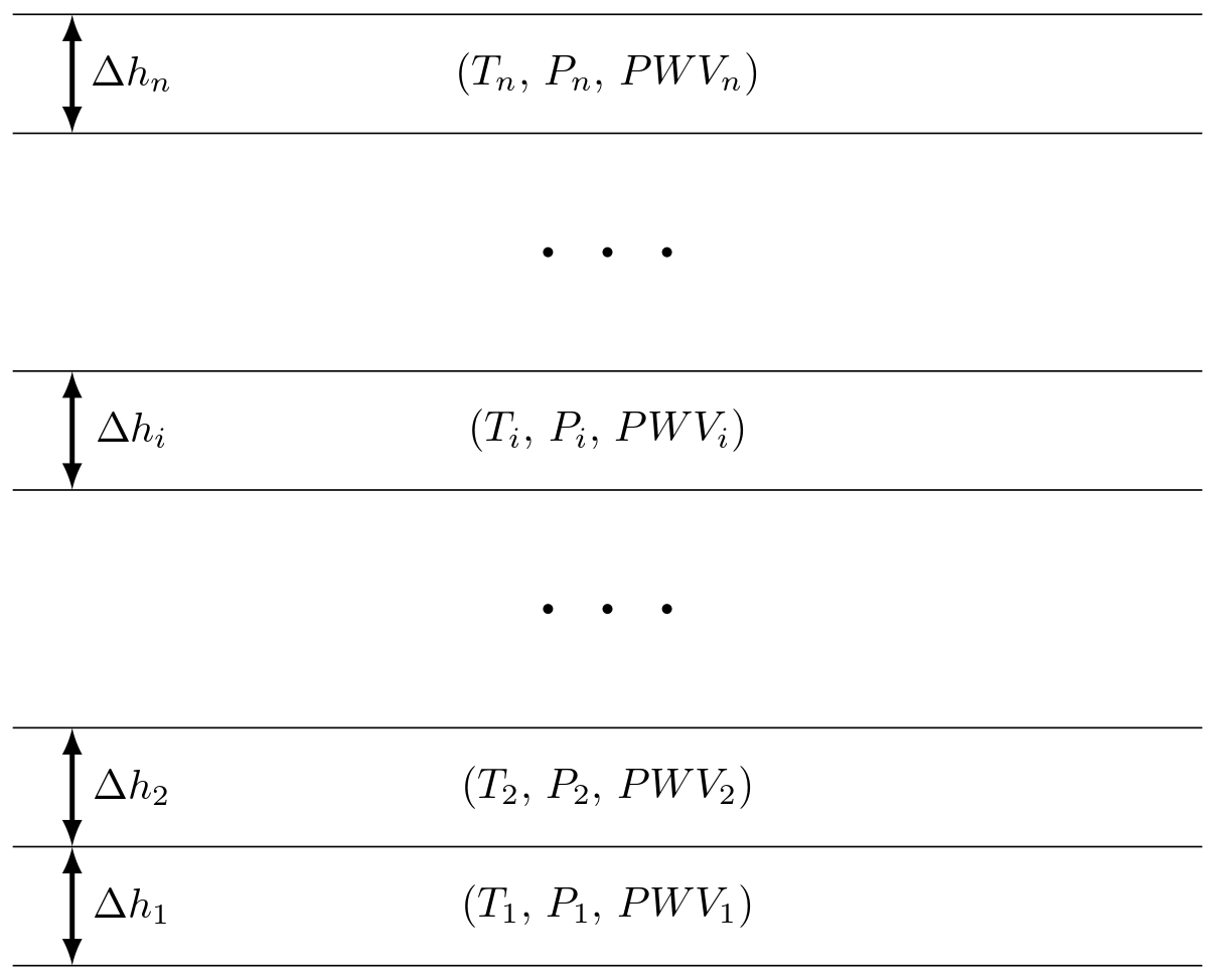
Neglecting all kinds of turbulent effects, the atmosphere can be treated using the plane-parallel model. According to this model, the atmosphere is divided into several overlapping homogeneous layers. Therefore each layer can be described by a group of parameters (called realization) that have the same value all over the layer. The most important parameters useful to describe the atmopsheric behaviour are temperature T, pressure P and precipitable water vapour PWV. Moreover each layer can be considered optically thin and in local thermodynamical equilibrium: as a consequence it is possible to solve the equation of the radiative transfer. Then the outcoming signal \(I_{out}\) is calculated as a function of the incoming one \(I_{in}\) as:
\[ I_\mathrm{out}(\nu)=B(\nu, T_\mathrm{phys,\;i})\cdot[1-e^{-\tau_i(\nu)}]+I_\mathrm{in}(\nu)\cdot e^{-\tau_i(\nu)} \]
where \(B(\nu, T_\mathrm{phys,\;i})\) is the black body at the physical temperature of the considered layer \(T_\mathrm{phys,\;i}\) and \(\tau_i(\nu)\) is the optical depth associated to the layer.
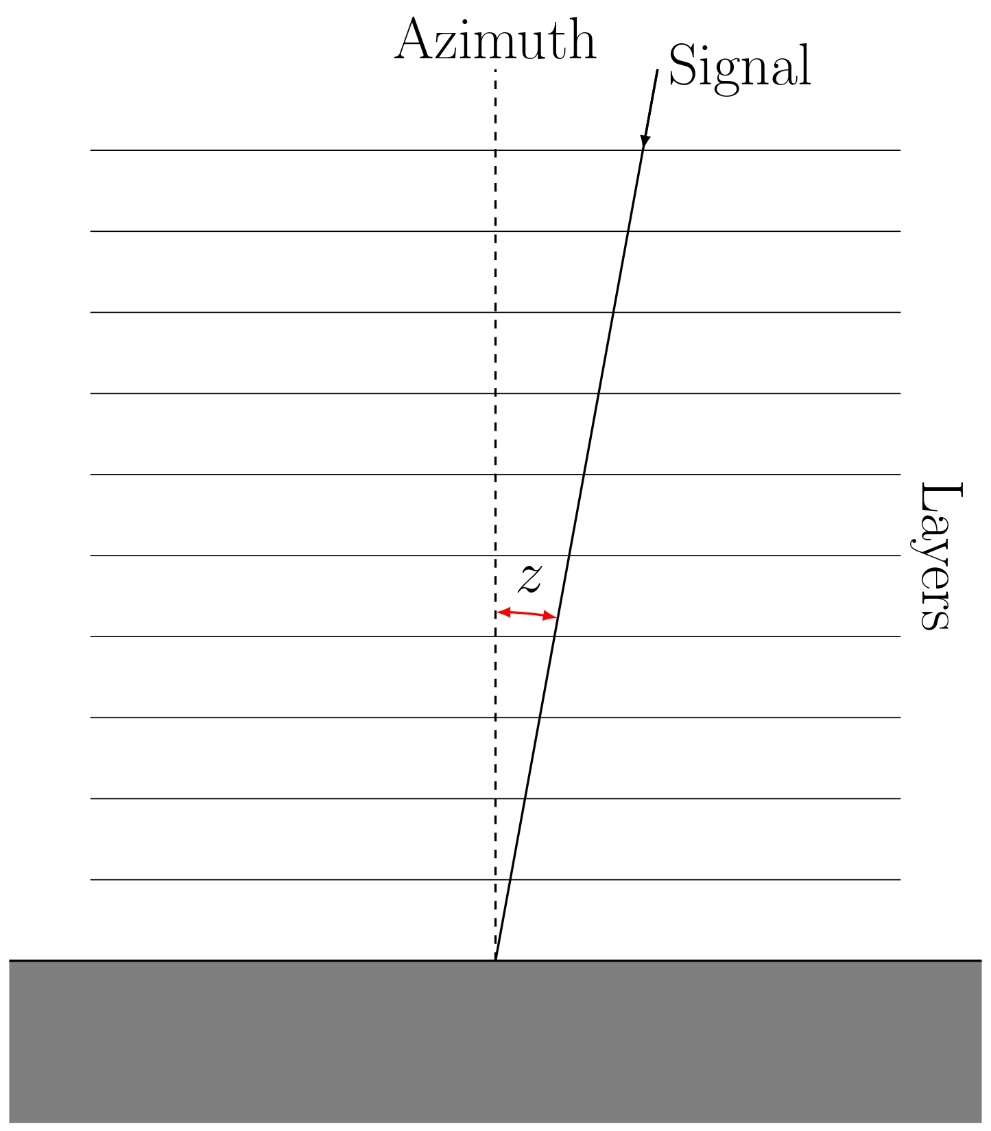
Iterating this kind of computation for all the layers composing the whole atmosphere, it is possible to find the signal observed from the ground. In fact it is assumed that the only signal entering the atmosphere from the top is the CMB (black body at \(2.73\;\mathrm{K}\)). As the atmosphere is treated as a sequence of homogeneous planes, the only dependence on the angle of observation (azimuth angle \(z\)) is:
\[ T_\mathrm{atm}(z)=\frac{T_\mathrm{atm, 0}}{\cos z} \]
where \(T_\mathrm{atm, 0}\) is the atmospheric brightness temperature at the zenith ( \(z=0\)).
In particular the statistical picture caught from the input data allows to perform the correlated sampling: in fact both temporal and intra-variables correlations are taken into accout. Thanks to this, this project can result in TODs of atmospheric relatizations. Therefore the resulting brightness temperatures maintain the correlated structures embedded in the data and could describe how the atmospheric signal evolves as time passes.
Notes
- This is a work in progress.